contours_m12.html

> restart;

CONTOUR DIAGRAMS

Graphs provide one way of visualizing functions of two variables. Another important way of visualizing such functions is by drawing their contour diagrams. With many options available, Maple can plot magnificent contour maps. Let's focus on the following interesting example. As in the first worksheet, we use classical Maple syntax to accomplish our goals. You can use context menus and plot builder if you prefer. In that case, make sure that you are in Worksheet Mode so all Maple commands are displayed.

Example 1. Examine the behavior of the function for g(x,y) = x^3 - 3x + y^3 - 3y, x,y near x = 0, y = 0. Create a contour map for the function.

We define the function

> g:=(x,y)->x^3-3*x+y^3-3*y;

(1)

Let's plot the function in a rectangle around x = 0 , y = 0. Finding a range around x=0, y=0 so that the graph shows clearly the behavior of the function around x=0, y=0 takes a bit of experimentation. One good range is x, y between -2 and 2. We choose this range. Also we lock in right away an orientation that gives us a good view of the surface.

> plot3d(g(x,y),x=-2..2,y=-2..2,axes=framed,orientation=[150,70]);

Plot

Rotate the surface to get a good sense of its shape! As you will learn later, the function has a local minimum, a local maximum, and two saddle points in the region.

Maple can create a contour diagram of the function with a simple command contourplot. The command, as well as the command display that we use below, is contained in the plots package. Hence, we load the package first and then ask for a contour map.

> with(plots):

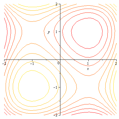
> contourplot(g(x,y),x=-2..2,y=-2..2);

Plot_2d

Maple drew a contour map. Note the characteristic appearance of the diagram near local extrema and near saddle points!

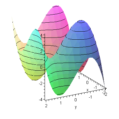
As you will see below, we can obtain a much fancier contour map by using a few additional options. Before we do it, let's consider how the contour diagram is created. As you know, a contour diagram is obtained by intersecting the graph of a function with horizontal planes corresponding to equally-spaced values of z, and projecting the resulting curves onto the xy-plane. Maple can illustrate very nicely how a contour diagram is created by plotting the graph of a function in patchcontour style. Let's do it for our function g(x,y).

> plot3d(g(x,y),x=-2..2,y=-2..2,axes=framed,style=patchcontour,orientation=[150,70]);

Plot

Here you see the contours before they are projected onto the xy-plane, that is, the intersections of the graph of the function with equally-spaced horizontal planes.

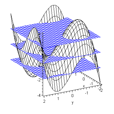
Maple can be used to illustrate how intersections themselves are obtained, as well. Let's draw the graph of g(x,y) and the horizontal planes z = -2, z = 0, z =2 in one coordinate system.

Note. Whenever you want to display more than one 3d graph in one coordinate system, you'd be better off using the display command, as we do below.

We define the four plots first. Some options that are common to all plots can be specified directly under the display command.

> p1:=plot3d(g(x,y),x=-2..2,y=-2..2,color=black):

> p2:=plot3d(-2,x=-2..2,y=-2..2,color=blue):

> p3:=plot3d(0,x=-2..2,y=-2..2,color=blue):

> p4:=plot3d(2,x=-2..2,y=-2..2,color=blue):

> display([p1,p2,p3,p4],axes=framed,style=hidden,orientation=[150,70]);

Plot

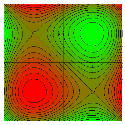
Next, we shall create a more sophisticated contour map of g(x,y) than the one above. We shall use the option that allows us to specify a sequence of contour levels and the coloring option that colors the map according to elevation. The syntax is as follows.

> contourplot(g(x,y),x=-2..2,y=-2..2,contours=[-3.5,-3,-2.5,-2,-1.5,-1,-0.5,0,0.5,1,1.5,2,2.5,3,3.5],filled=true,coloring=[green,red]);

Plot_2d

The redder shades on our map correspond to higher elevations. The green shades correspond to lower elevations. Hence, we see clearly: there is a high hill in the third quadrant, a low crater in the first quadrant, and two saddle-shaped areas in the second and fourth quadrants. The commands responsible for coloring the map are filled=true and coloring=[green,red]. Needless to say, you can replace the two colors with any other colors you prefer. Also, you can use the coloring commands without specifying contour levels and vice-versa.

Remark. If you want to obtain a contour map that allows you to read clearly the steepness of slopes and the shape of a surface, you should always take equally-spaced values for level curves, as we did in the above example. When we do this, closely-spaced contours on a contour map indicate steep increase or decrease in elevation, while contours far apart indicate mild slopes.

Level Surfaces

As you know, contour maps are useful for representing functions of two variables f(x,y). Each contour is a curve on the (x,y)-plane along which the function has constant values f(x,y)=c. The analogue of a contour in the case of a function f(x,y,z) of three variables is a level surface. A level surface for f(x,y,z) and a given constant c is the surface in the (x,y,z)-space for which f(x,y,z) is equal to c, that is, the surface with the equation f(x,y,z)=c. Level surfaces are not as easy to visualize as contours, but Maple can be helpful here, too. To plot a few level surfaces for a given function, we use the command implicitplot3d contained in the plots package. The command plots surfaces defined by (x,y,z)-equations.

Example 2. Consider the function f(x,y,z) = - x^2 + y^2 + z^2. Plot its level surfaces corresponding to the level values 1/10 and 2. Display the two surfaces in one coordinate system.

> f:=(x,y,z)->-x^2+y^2+z^2;

(2)

We shall label the two plots corresponding to the two surfaces by s1, s2, and then display them together using the display command. We shall use the style=wireframe option that allows us to see inside each surface. Note that for implicit plots you have to specify ranges for all variables x, y, and z. Sometimes you have to experiment a little in to find ranges that give you a good looking plot.

> s1:=implicitplot3d(f(x,y,z)=1/10,x=-2..2,y=-2..2,z=-2..2,style=wireframe,color=black):

> s2:=implicitplot3d(f(x,y,z)=2,x=-2..2,y=-2..2,z=-2..2,style=wireframe,color=blue):

> display([s1,s2],axes=framed,scaling=constrained);

Plot

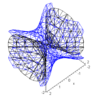You see two hyperboloids, one contained inside the other. These are two level curves for the function f(x,y,z).

Homework Problems

Note. If you restart Maple before doing your homework, do not forget to reload the "plots" package: with(plots): .

If a problem calls for explanations, be sure to type clear, complete explanations.

In the problems below, you are expected to create only one color-filled contour map. This is to avoid running out of memory and cut down on printing time. If your computer has plenty of memory and your printer is fast , you can do all contour maps as color-filled.

Problem 1. Consider the function

m(x,y) = exp( - (x^2 + 3*y^2)) .

(a) Draw the graph of the function in the patchcontour style. Choose a range for x and y not too large, so that the shape of the function near x = 0, y=0 is clearly visible and the graph is not too choppy, but large enough so that the global behavior of the function is evident. What symmetries does the graph have? Describe the shape and the behavior of the graph in your own words.

(b) Create a contour map and explain how it reflects the shape of the graph. Do not use filled=true option in this example.

Problem 2. Recall the string from the previous worksheet that is pegged along the x-axis with the endpoints at x=0 and x=1. You pluck the string in a certain way so it vibrates according to the formula

v(x,t) = cos(t) sin( 2 * Pi * x ) ,

where t is the time, in milliseconds, x the horizontal coordinate of a point on the string. v(x,t) denotes the vertical displacement of the point x at time t. (We are assuming that each point vibrates only in the vertical direction.)

(a) Create a color-filled contour map for v(x,t) for x between 0 and 1, and t between 0 and 7.

(b) Explain how the map reflects the motion of the string.

Problem 3. Consider the function

h(x,y,z) = x^2 + 2y^2 + z^2 .

Plot, in one coordinate system, the two level surfaces for the function corresponding to h(x,y,z)=1 and h(x,y,z)=2.

Updated for Maple 12 by B.Kaskosz, 2009.